Data Loading

A key challenge in quantum computing applications — such as quantum machine learning, finance, and optimization — is efficiently encoding classical data into quantum states. While loading data into the amplitudes of a quantum state allows one to load

2^{NumQubits}

values, the standard circuits to prepare such states may require an exponentially large number of operations in number of qubits, making it impractical.

Haiqu’s data loading methods allow encoding of an arbitrary data into the amplitudes of the quantum state. They are particularly useful for applications in quantum simulation, machine learning, quantum optimization, solving differential equations and others.

Loading an arbitrary 1D data vector

Here we introduce one of the loading procedures available in Haiqu SDK: Vector Loading allows to load a vector (1D array) of classical data directly into the amplitudes of a quantum state, producing compact, linear-in-depth circuits.

The input vector is a real- or complex-valued one-dimensional vector, which contains the values to be encoded in the amplitudes. Vector Loading automatically adjusts to the closest minimal necessary number of qubits and normalizes the data. The current supported maximum size of the vector is

2^{20} =1,048,576

Haiqu SDK allows you to prepare custom quantum states from classical data vectors by calling haiqu.vector_loading(...).

job = haiqu.vector_loading(
    name="Data Loading Circuit",    # Name
    data=data_vector                # 1D list with values 
    )

gate = job.result()     # a HaiquCircuitGate, encapsulating state preparation circuit
fidelity = job.quality  # fidelity of the state preparation circuit

vector_loading , like all other Haiqu’s data loading routines, returns a HaiquCircuitGate object, which is an abstract Qiskit circuit instruction and can be substituted into user’s circuits at any place just like other standard gates. HaiquCircuitGate will be unpacked into elementary gates, performing state preparation, at transpilation time internally. All data loading jobs report a global quantum state fidelity of the synthesized circuit, that is, an overlap with a quantum state, defined by the input data, and a state, produced by a generated quantum circuit, is computed. It allows to access the quality of the result and possibly tune the synthesis parameters.

Loading an arbitrary state at utility scale

Amplitude encoding has a scaling limitation: it is not possible to explicitly store in a classical memory a state vector for arbitrary large systems, therefore it is not possible to apply Vector Loading to them. To alleviate this problem we use the Matrix Produce State (MPS) representation of a wave-function. It is written as a sequence of matrices (tensors) which, when contracted, restore the original state vector. Setting a limit on sizes of such matrices allows to store a “compressed” version of a quantum state at large scales, inaccessible by other means. MPS is a popular method for large scale simulations, however can successfully (without large errors) represent only states with low entanglement. Haiqu SDK contains the MPS Loading method, which can generate state preparation circuits at utility scale. The method takes a MPS as an input and supports two MPS formats: the standard MPS (written as sequence of site tensors) and the Vidal form (where in addition a sequence of bond tensors appears). Using MPS Loading is very simple:

job = haiqu.mps_loading(
    name="Data Loading Circuit",    # Name
    mps=mps                         # input Matrix Product State
    )

The method is particularly useful when the user wants to prepare large scale custom state on a quantum computer, for example, when switching from a classical tensor network simulation to a quantum simulation of some evolution.

Loading multidimensional data

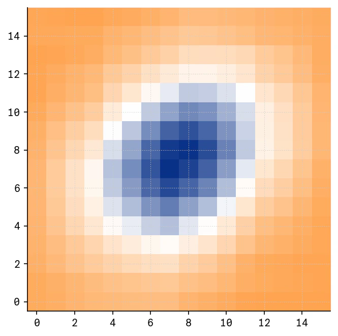
In many applications, the input data is naturally represented as a multidimensional array. In the following example we show how to load a custom 2D distribution. First, we prepare a 2D array with multivariate normal distribution on a rectangular

16\times 16

grid:

import numpy as np
from scipy.stats import multivariate_normal
# preparing a grid
x = np.linspace(-3, 3, 16)
y = np.linspace(-3, 3, 16)
grid = np.stack(np.meshgrid(x, y), axis=-1)  # 2D grid 16x16

# 2D Normal distribution on the grid
data = multivariate_normal([0, 0], [[1, 0.3], [0.3, 1]]).pdf(grid)
# in applications square roots of probability distributions are often used
data = np.sqrt(data)

Since haiqu.vector_loading(...) expects a one-dimensional input vector, the data array should first be flattened:

data = data.ravel()  # convert to 1D array

The data can now be loaded with haiqu.vector_loading(...):

job = haiqu.vector_loading(data, name="Multidimensional distribution")
gate = job.result()  # a HaiquCircuitGate, encapsulating state preparation circuit

Using numpy.ravel() will naturally order the values in such a way that Vector Loading will use blocks of consecutive qubits for each data dimension (see example below). Such representation often expected in quantum applications.

In this example, 8 qubit state will be created, where first 4 qubits will correspond to the Y axis, and the last 4 qubits will correspond to the X axis. The correctness of the encoding can be verified on e.g. a statevector simulator. In our example we recover the original 2D Normal distribution, which we plot below:

# creating a state preparation circuit
# using the constructed HaiquCircuitGate
qc = QuantumCircuit(8)
qc.compose(gate, inplace=True)

# running exact statevector simulator to access amplitudes
sv = haiqu.statevector_run(qc).result()[0]

# plotting the loaded 2D distribution
plt.imshow(np.real(np.resize(sv, (16, 16))), origin="lower")

Vector Loading specifications

Parameter	Details
Number of qubits	Up to 20 qubits
Input data	1D vector
Data type	Real and complex values
Data size	Up to ~1M features in the vector
Runtime	0.5–2 minutes
Runtime scaling	Linear scaling with number of qubits
Circuit size (gates count)	O(n), n = number of qubits
Circuit depth	O(n/2), n = number of qubits
Circuit connectivity	Linear
Other circuit properties	- No mid-circuit measurements - Only CNOT and single-qubit rotation gates - No ancilla qubits - No post-selection required in state preparation
Returned metrics	Quantum state fidelity is returned for the ideal state prepared by the circuit

Matrix Product State Loading specifications

Parameter	Details
Number of qubits	Up to 1000 qubits
Input data	MPS in standard or Vidal form
Data type	Tensors with real and complex values
Bond dimension	Up to 64
Runtime	0.5–2 minutes
Runtime scaling	Linear scaling with number of qubits
Circuit size (gates count)	O(n), n = number of qubits
Circuit depth	O(n/2), n = number of qubits
Circuit connectivity	Linear
Other circuit properties	- No mid-circuit measurements - Only CNOT and single-qubit rotation gates - No ancilla qubits - No post-selection required in state preparation
Returned metrics	Quantum state fidelity is returned for the ideal state prepared by the circuit

​Loading an arbitrary 1D data vector

​Loading an arbitrary state at utility scale

​Loading multidimensional data

​Vector Loading specifications

​Matrix Product State Loading specifications

Loading an arbitrary 1D data vector

Loading an arbitrary state at utility scale

Loading multidimensional data

Vector Loading specifications

Matrix Product State Loading specifications