

state_compression function is an approximate compilation method extending the depth of the circuit, which can be run on noisy hardware. It automatically adjusts the compression parameters to achieve the best performance by taking into account the device’s characteristics, including noise and topology.
Linear topology compression
To compress a circuit using idealized linear topology you simply create a state compression jobquality metric is a fidelity-like metric, which Haiqu internally computes in the end of the compression to quantify circuit approximation quality on a noiseless device. Unlike quantum state fidelity it is scalable and does not vanish with increasing the systems size, meanwhile it is highly correlated with the observables precision. As a rule of thumb you can treat its values as follows:
Haiqu’s compression utilizes the device’s noise profile to ensure the best results on actual hardware. Default noise settings correspond to IBM’s Heron R2 device and can be changed by modifying
noise_profile parameter (see below). State compression function can trade-off theoretical approximation on an ideal device for more compact circuits that perform better on real quantum hardware.qiskit.circuit.random.random_circuit.
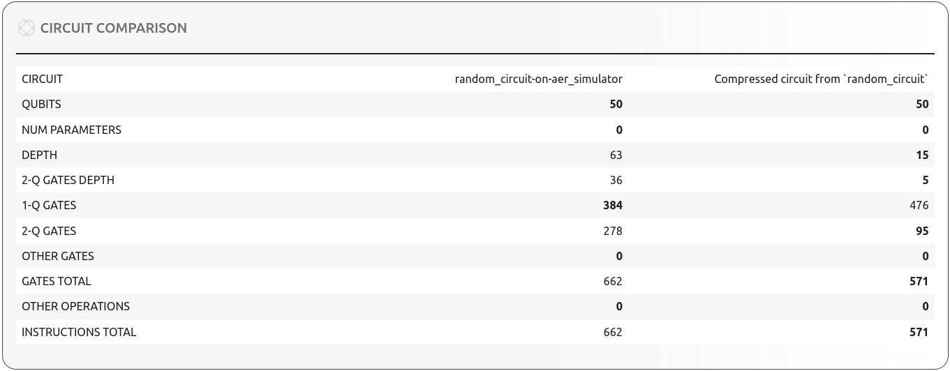
Device topology-aware compression
To use device topology-aware compression, use thestate_compression_2d method. For example:
state_compression_2d is currently limited only to devices with heavy-hex connectivity.Measuring the compressed circuit
job.result() returns a CircuitModel, not a plain QuantumCircuit or HaiquCircuitGate.
Local circuit.depth() and gate counts are misleading on opaque gates; transpile with Haiqu and
read circuit analytics on the returned CircuitModel:
Parameters
circuit– the quantum circuit whose action on all-0 state is to be compressed.compression_level– defines the compression level. Increased compression level will lead to larger part of the input circuit being compressed. Three options are available:low– this setting is best used for already shallow input circuits or very low noise levels;balanced– the default setting gives the best performance for most circuits and noise profiles;high– this setting may sometimes yield better results for very deep circuits.
noise_profile– sets the noise profile to which the function adjusts the compression algorithm. Used to automatically set the approximation level. Currently available options are"ibm_eagle_r3","ibm_heron_r1","ibm_heron_r2"(used by default),"ibm_heron_r3","iqm_garnet"and"iqm_emerald".fine_tuning– uses classical resources to further improve the compressed circuit. Three options are available:disabled– no fine-tuning performed, the lowest latency;low– default, best balance between speed and accuracy;heavy– improved circuit accuracy, but time-intensive.
approximation_level– an integer-valued parameter influencing circuit complexity. Larger values improve the noiseless quality metric, but may degrade noisy performance. Defaults to None, which corresponds to auto-selection using the provided noise profile. Can be set to any value from 1 (very weak approximation) to 8 (very high approximation). Larger approximation level values lead to slower fine-tuning.deviceordevice_id(only forstate_compression_2d) – target device for the compression.
haiqu.state_compression and haiqu.state_compression_2d.
State Compression Specifications
State Compression 2D Specifications
*runtime can vary for different circuit classes of the same size