| Property or Function | Description |
|---|---|
haiqu_circuit.analytics | Provides ALL raw metrics data, represented as Python objects. |
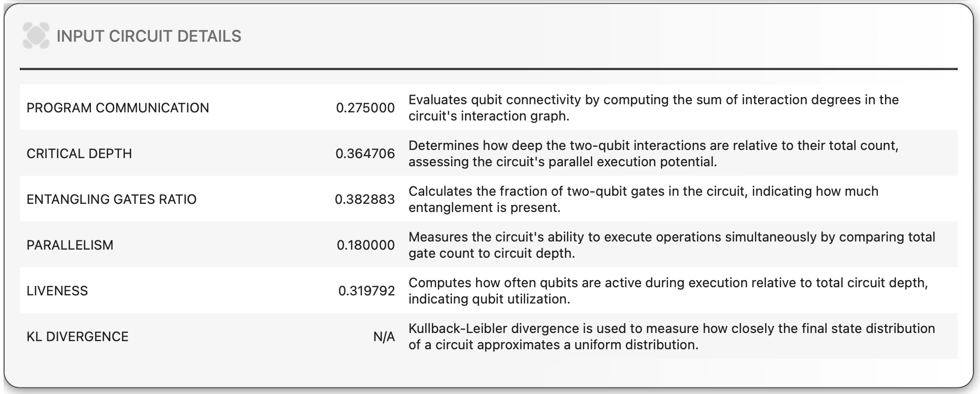
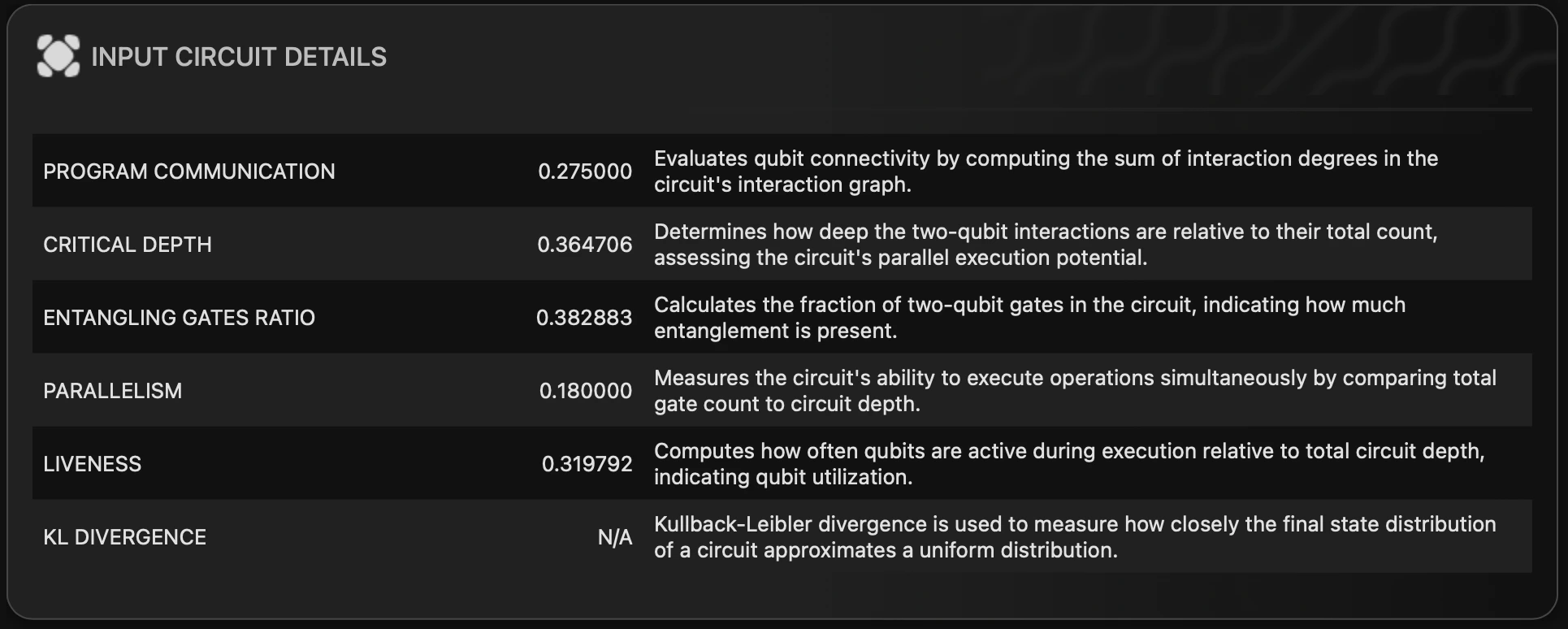
haiqu_circuit.core_metrics() | Renders a widget that displays a table of core analytics metrics. |
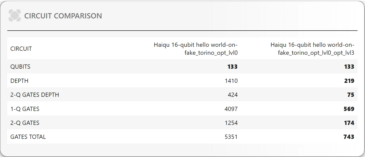
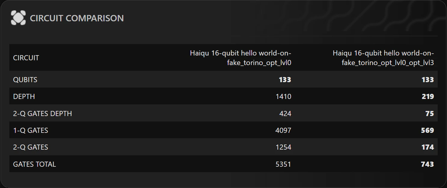
haiqu_circuit.compare_metrics() | Renders a widget with a comparison table of core analytics for provided circuits. |
haiqu_circuit.compute_advanced_metrics() | The advanced metrics are computed on demand, to invoke the computation, call this method first. |
haiqu_circuit.advanced_metrics() | Renders a widget that displays a table with advanced quantum circuit metrics. |
haiqu_circuit.compute_evolution() | The circuit evolution data are computed on demand, to invoke the computation, call this method first. |
haiqu_circuit.evolution | Provides raw metrics data for the circuit, as the circuit is traversed, represented as Python objects. |
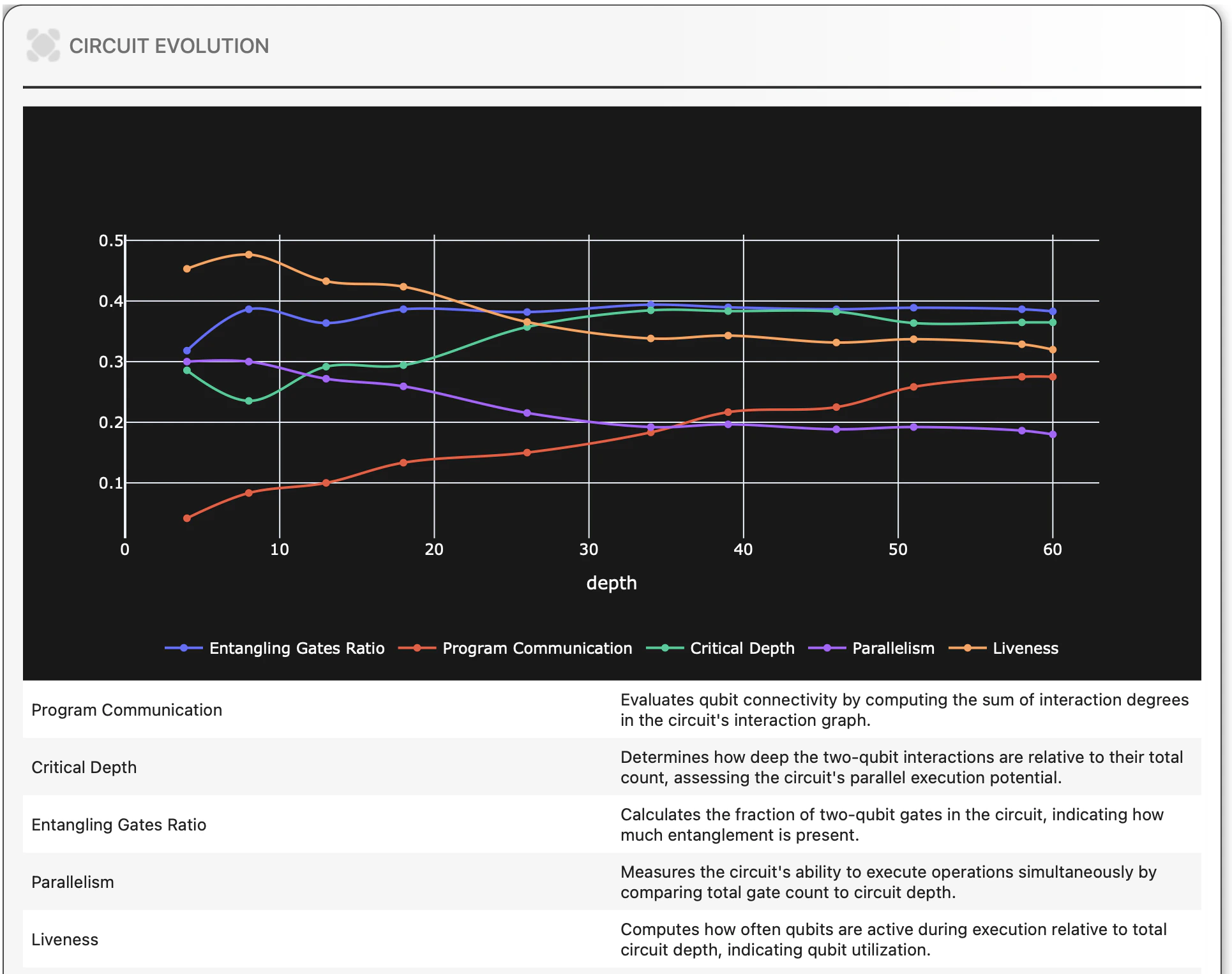
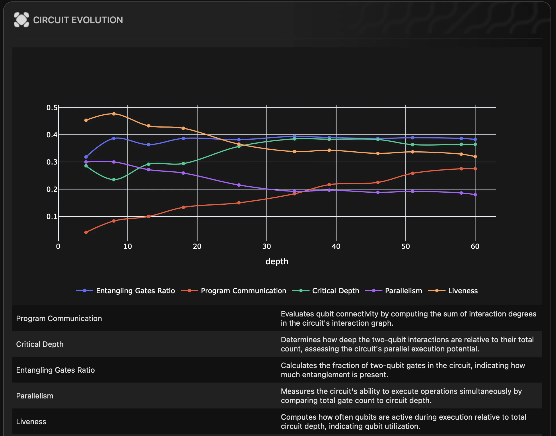
haiqu_circuit.draw_evolution() | Generates a plot showing the evolution of key circuit metrics as the circuit is traversed. The original circuit is divided gate-by-gate or into slices, based on the initial depth. Metrics are calculated for each slice. |
haiqu_circuit.draw_radar() | Renders a widget displaying the radar (wind-rose) plot. |
haiqu_circuit.draw_gate_diversity() | Renders a widget showing the number of different gates in the circuit. It has two modes: original and normalized to basis gates. The basis_gates=True option will display the normalized (transpiled to basis gates set RX, RY, RZ and CX) view for gate diversity. |
haiqu_circuit.draw_liveness_per_qubit() | Renders a widget displaying the liveness per qubit plot. The liveness metric reveal the frequency of qubit activity during execution in relation to the total circuit depth, indicating qubit utilization. |
haiqu_circuit.draw_correlation_matrix() | Renders a normalized interaction matrix (heatmap) that quantifies how frequently each pair of qubits participates together in two-qubit gates within a given quantum circuit. |
help=True option. Whenever possible, the widget displays a column to provide assistance for each metric. Data can be exported in formats including JSON, CSV, or used in Pandas for further analysis.
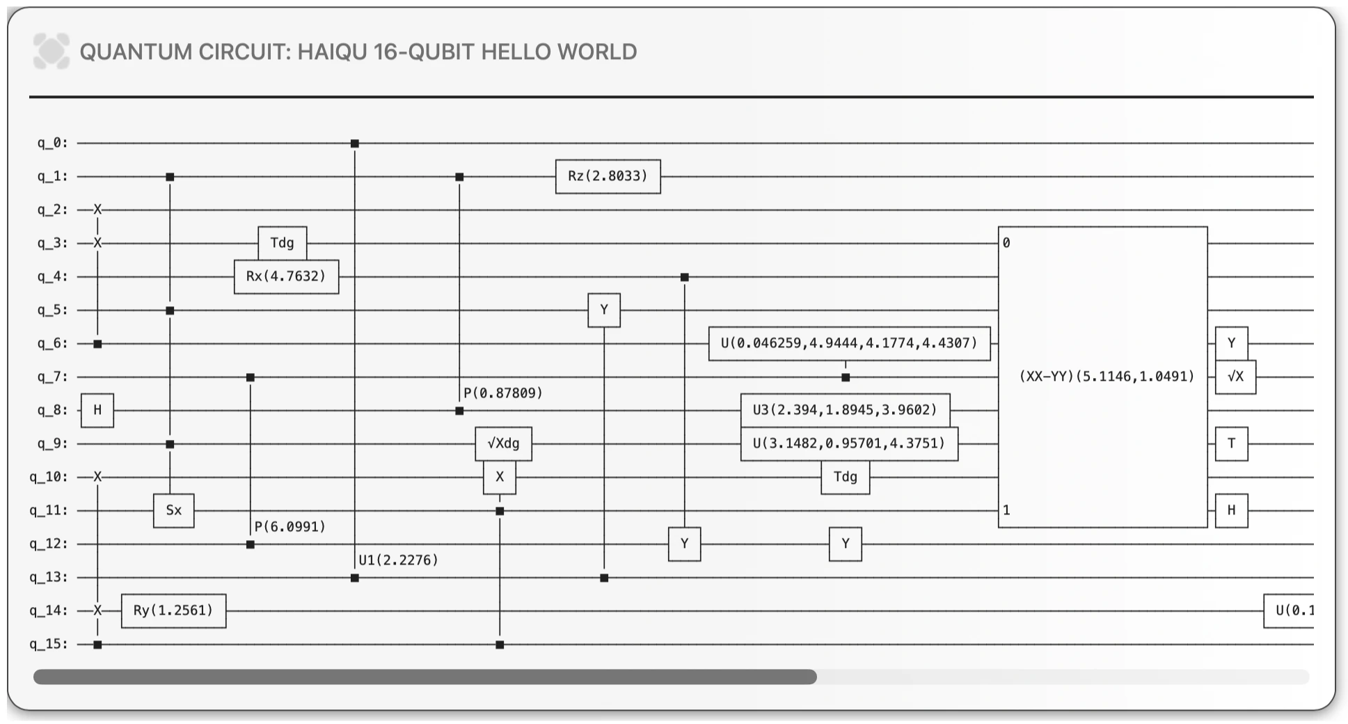
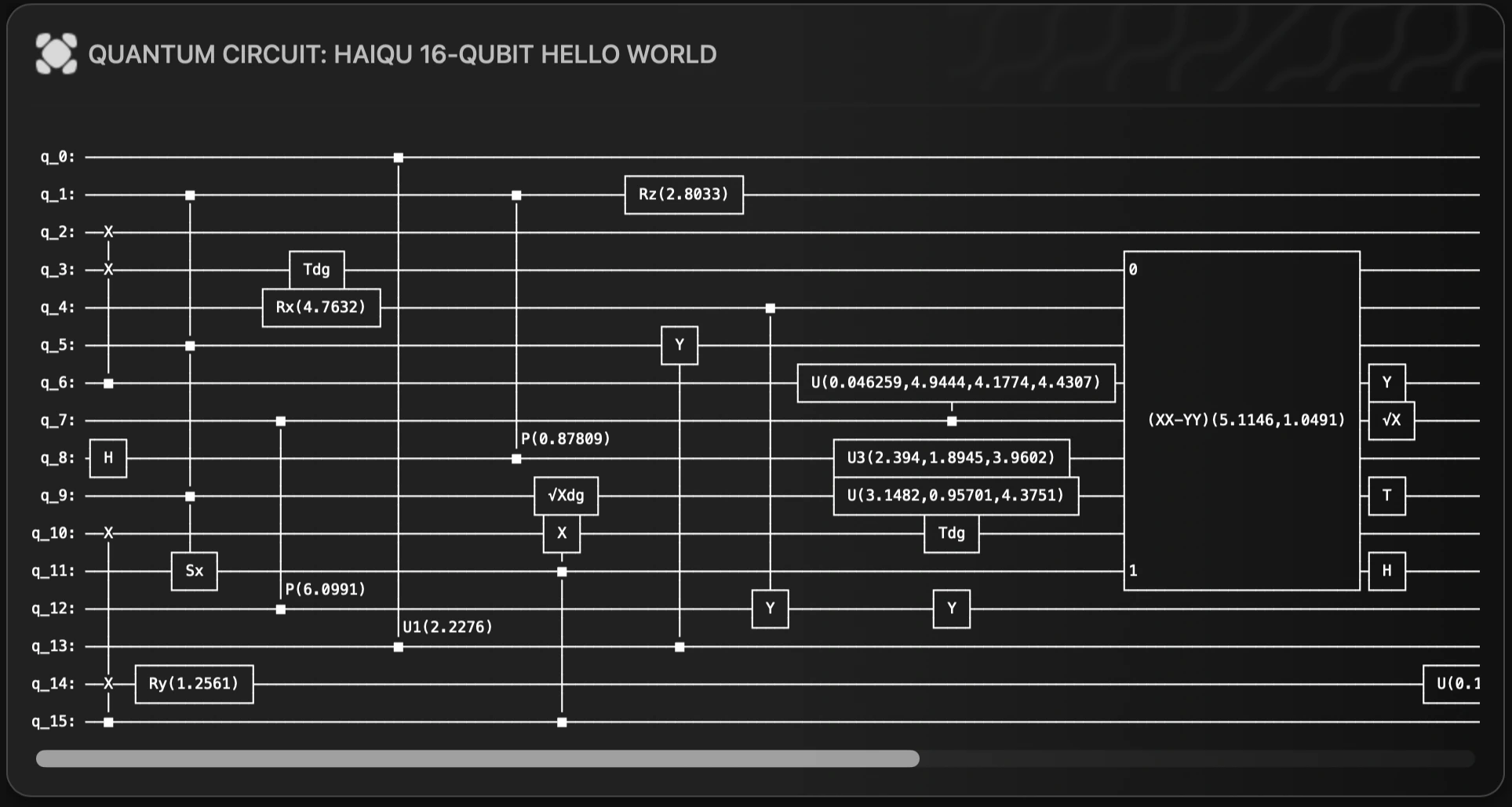
Let’s start by defining an example quantum circuit, then display it:
haiqu.log() method. This computes the complete set of quantum metrics using the Haiqu API and returns them in a single metadata object.
Let’s submit our circuit to the Haiqu quantum backend for analysis:
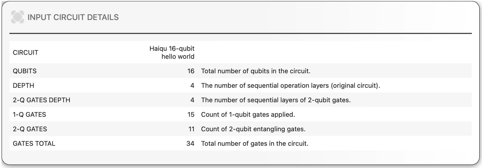
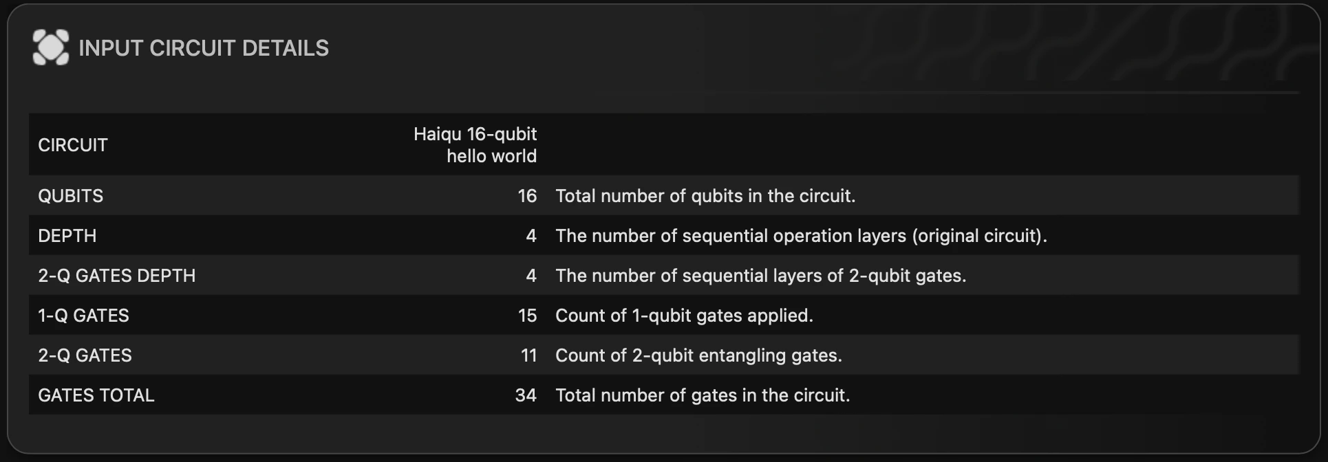
Basic analysis
Before executing a quantum circuit, it is crucial to assess its fundamental properties to ensure feasibility and compatibility with available simulators or hardware. This step helps determine circuit size, gate composition, and whether it contains custom or unsupported operations. By analyzing these factors, users can make informed decisions about device selection, potential optimizations, and whether additional modifications are needed before execution. The circuit’s basic metrics are displayed usingcore_metrics:
Advanced analytics
The advanced metrics are computed on demand; to invoke the computation, callcompute_advanced_metrics() first. Then, to display the advanced circuit metrics, call advanced_metrics():
Evolution of the circuit
Generate a plot showing the evolution of key circuit metrics during simulated execution of the circuit. The original circuit is divided into slices, and metrics are calculated for each slice, providing insights into changes in connectivity, depth of two-qubit interactions, degree of entanglement, and concurrent operation performance. The evolution of metrics is computed on demand; to invoke the computation, callcompute_evolution() first. Then call draw_evolution(metric) to render the plot. The metric parameter set according to which metric to plot the evolution. Possible values are depth, gates_1q, gates_2q, gates_total. Defaults to depth.
Comparing circuits
The functionhaiqu.compare_metrics could be useful for comparing the different circuits or the circuit built with different parameters. It could compare up to N different circuit and provide a table-like widget.
Circuit-Analytics.ipynb notebook in Haiqu Lab.