> ## Documentation Index
> Fetch the complete documentation index at: https://docs.haiqu.ai/llms.txt
> Use this file to discover all available pages before exploring further.

# Distribution Loading

> Load distributions with compact circuits at record scales

A key challenge in quantum computing applications — such as quantum machine learning, finance, and optimization — is efficiently encoding classical data into quantum states.

In this tutorial, we'll load a classical probability distribution (like the normal distribution) into a quantum state, which is a core primitive for various financial and simulation applications.

<Tip>
  * **Goal**: Encode a probability distribution into a quantum state such that measurement outcomes follow the target distribution.
  * **Use Case**: Financial modeling, probabilistic simulations, quantum generative models.
  * **How it works**: The square root of the distribution (e.g., Gaussian) is encoded in quantum amplitudes via state preparation circuits.
</Tip>

Haiqu SDK offers a simple function to load over 100 distributions supported by [scipy.stats](https://docs.scipy.org/doc/scipy/reference/stats.html#continuous-distributions) library. For example, loading a Normal distribution into the quantum state can be done by running the following function that initializes a data loading job:

```python theme={null}
job = haiqu.distribution_loading(
  name=f"DL norm {num_qubits}q",        # Name
  num_qubits=num_qubits,                # Number of qubits
  distribution_name="norm",             # Distribution to load
  interval_start=-3, interval_end=3,    # Interval over which to load
  num_layers=2                          # Precision parameter 
  )
```

The corresponding state preparation gate is returned by calling `job.result()`the job result:

```python theme={null}
data_loading_gate = job.result()  # a HaiquCircuitGate, encapsulating state preparation circuit
fidelity = job.quality            # fidelity of the state preparation circuit
```

Above `fidelity` quantifies the overlap between a wavefunction generated by the synthesized circuit and the exact discretized input distribution, computed as [quantum state fidelity](https://en.wikipedia.org/wiki/Fidelity_of_quantum_states).

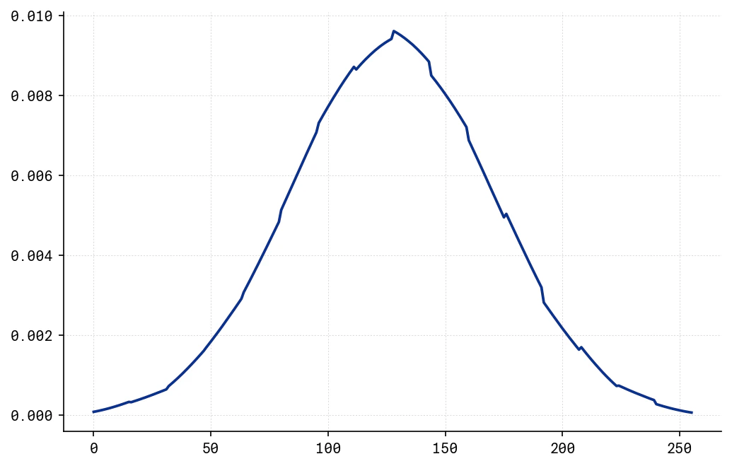
The quality of the obtained data loading circuit can be visually verified using e.g. statevector simulation. For the Normal distribution example using `num_qubits=8` we obtain the following result:

```python theme={null}
qc = QuantumCircuit(num_qubits)
# add the data loading gate to the circuit
qc.compose(data_loading_gate, inplace=True)

# run exact simulation
sv = haiqu.statevector_run(qc).result()[0]

# plot probabilities
plt.plot(np.square(np.abs(sv)))
```

<Frame>
  <img src="https://mintcdn.com/haiqu/DjRJlqQlLMCYZfXw/images/1d_normal_example.png?fit=max&auto=format&n=DjRJlqQlLMCYZfXw&q=85&s=f9ef31259a345a25123e20b2bfe33937" alt="Image" width="1035" height="659" data-path="images/1d_normal_example.png" />
</Frame>

The required parameters of the `distribution_loading` method are:

* `distribution_name:` name of the statistical distribution from `scipy.stats`.
* `interval_start` and `interval_end`: the boundaries of the interval over which the distribution will be discretized before loading into the quantum state.
* `num_qubits` : the number of qubits used, which sets the discretization resolution.

Additionally, the user can control advanced parameters, such as:

**Distribution Hyperparameters (Optional, follows SciPy's API)**

* `loc` (default: 00) → The location/mean of the distribution.
* `scale` (default: 11) → Scale or spread, often linked to variance.
* `shape` parameters → Distribution-specific extra parameters. Check SciPy docs for details.

**State Preparation Hyperparameters (Optional)**

* `num_layers` (default: 11) → Number layer in the data loading circuit. More layers = better approximation of data or distribution, but more gates.
* `truncation_cutoff` (default: `1e-6`) → A threshold for cutting off low-entanglement gates. Set to `None` or `0` for no truncation (full entanglement retained).

## Distribution Loading Specifications

| **Parameter**                  | **Details**                                                                                                                                                            |
| :----------------------------- | :--------------------------------------------------------------------------------------------------------------------------------------------------------------------- |
| **Number of qubits**           | Up to 1000 qubits                                                                                                                                                      |
| **Number of distributions**    | 107 different classes of distributions are supported. Check SciPy docs for details.                                                                                    |
| **Runtime**                    | 1–15 seconds                                                                                                                                                           |
| **Runtime scaling**            | Linear scaling with number of qubits                                                                                                                                   |
| **Circuit size (gates count)** | O(n), n = number of qubits                                                                                                                                             |
| **Circuit depth**              | O(n/2), n = number of qubits                                                                                                                                           |
| **Circuit connectivity**       | Linear                                                                                                                                                                 |
| **Other circuit properties**   | - No mid-circuit measurements <br /> - Only CNOT and single-qubit rotation gates <br /> - No ancillary qubits <br /> - No post-selection required in state preparation |
| **Returned metrics**           | Quantum state fidelity is returned for the ideal state prepared by the circuit                                                                                         |